Single and Multi-objective Parameter Estimation of a Military Personnel System via Simulation Optimization

by Lee Alan Evans, Ki-Hwan G. Bae, and Arnab Roy (University of Louisville)

As presented at the 2017 Winter Simulation Conference

A discrete event simulation model is developed to represent a forced distribution performance appraisal system, incorporating the structure, system dynamics, and human behavior associated with such systems. The aim of this study is to analyze human behavior and explore a method for model validation that captures the role of subordinate seniority in the evaluation process. This study includes simulation experiments that map black-box functions representing human behavior to simulation outputs. The effectiveness of each behavior function is based on a multi-objective response function that is a sum of squared error function measuring the difference between model outputs and historical data. The results of the experiments demonstrate the utility of applying simulation optimization techniques to the model validation phase of simulation system design.

Background

The United States Army used a variety of techniques to decrease the number of active duty Army personnel from over 566,000 in 2010 to below 470,000 in 2016. These techniques included involuntary separation boards, early retirement boards, decreased accessions, decreased reenlistment opportunities, and decreased promotion rates. Central to each of these force shaping mechanisms, with the exception of decreased accessions, was the analysis of performance appraisals.

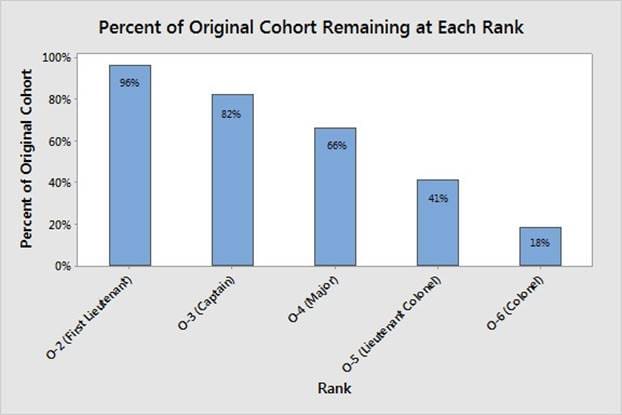
Performance appraisals are of significant importance in the officer ranks due to the Defense Officer Personnel Management Act of 1980 (DOPMA). This act, passed by Congress on December 12, 1980, dictates the number of officers as a function of the overall Army personnel strength level, but more importantly,   it codifies the up-or-out promotion system (Rostker et al. 1993). The up-or-out promotion system was designed such that officers are evaluated by promotion boards and if selected, move through the ranks in cohorts, generally determined by years of service as an officer. Furthermore, any officer twice passed over for promotion to the next rank is forced to leave the service. The only exception to the separation mandate is a provision allowing for selective continuation for select officers, with the intent that it would be used sparingly. The up-or-out promotion system facilitates the rank structure shown in Figure 1, which was also set forth in DOPMA.
One of the ranks most affected by the drawdown was the rank of lieutenant colonel,  which went  from a promotion rate of over 91% in 2006 to a promotion rate of just 60.2% in 2016.  An analysis of    the promotion board results shows that the identified percentiles on evaluations are the best indicator of whether an officer was promoted. The United States Army officer performance appraisal system is a forced distribution system that uses a relative comparison of officers within a rating pool and forces raters to give top evaluations to less than 49% of their subordinates (Department of the Army Headquarters 2015). Further analysis of the promotion board results shows that seniority plays a significant role in whether or not an officer receives a top evaluation. However, the function used by raters to sort and evaluate subordinates is unknown (black-box) and noisy due to raters’ individual prioritization of seniority.

Related Literature

Previous work in manpower modeling is extensive.  For the purpose of this simulation system design,   we reviewed manpower planning methods, performance appraisal systems, talent management, simulation optimization, and model validation.

Bartholomew, Forbes, and McClean (1991) define manpower planning as “the attempt to match the supply of people with the jobs available for them”. Wang (2005) classifies operations research techniques applied in manpower planning into four branches: optimization models, Markov chain models, computer simulation models, and supply chain management through System Dynamics. Hall (2009) notes that existing literature on manpower planning falls under one of three main topics: dynamic programming, Markovian models, and goal programming. While the lists are neither exhaustive nor mutually exclusive, we classify existing techniques into the categories of optimization, Markov, and simulation models.

Early examples of optimization models include dynamic programming models that provide a framework for human resource decision making (Dailey 1958, Fisher and Morton 1968). A more recent dynamic programming application is that of Ozdemir (2013), providing an analytic hierarchy processing order for personnel selection. Bres et al. (1980) and Bastian et al. (2015) provide goal programming models to analyze officer strength and occupational mix over a finite time horizon. Kinstler et al. (2008) uses a Markovian model for the U.S. Navy Nursing Corps to determine the optimal number of new recruits to resolve the issue of overstaffing at lower ranks in order to meet requirements at higher ranks. While Markov models can be used as stand-alone models, they are more commonly incorporated into larger optimization models (Hall 2009, Zais 2014). Lesinski et al. (2011) and McGinnis, Kays, and Slaten (1994) are examples of simulation used for manpower modeling. The simulation construct developed by Lesinski et al. (2011) is used to determine whether the timing and duration of officer initial training supported a new Army unit readiness model. Similarly, McGinnis, Kays, and Slaten’s (1994) discrete event simulation model analyzes the feasibility of proposed personnel policies requiring a minimum amount of time in key assignments. What is germane to all of the existing methods is that they focus on meeting requirements in aggregate form. That is, the models estimate accessions and lateral entry requirements based on historical attrition, promotions, and forecasted growth. Very little attention is given to modeling the systems that identify and select the most qualified individuals to fill requirements rather than the binary measurement of whether a position is occupied or vacant.

Wardynski, Lyle, and Colarusso (2010) define U.S. Army officer talent as the intersection of individual knowledge, skills, and behaviors. Dabkowski et al. (2010) note that measuring officer talent is largely conceptual, but actual measurements are not necessary to analyze the talent retention impacts of policy. Their model uses a normally-distributed talent score to analyze the impact of multiple attrition patterns on the talent of senior leadership. Wardynski, Lyle, and Colarusso (2010) show that commissioning sources with the most stringent screening requirements produce higher performing officers in the senior ranks, adding credence to the Dabkowski et al. (2010) treatment of talent as a static, innate value.

Performance appraisal systems are known to have inherent bias and error. Examples of bias and error within performance appraisal systems are difficult to quantify, but include: raters evaluate more generously (leniency) or harshly (severity) than subordinates deserve, raters forming positive (halo) or negative (horn) opinions around a limited number of criteria, recent performance weighing heavily (recency), raters elevating subordinate rating to make themselves look better (self-serving), and rating subordinates relative to each other rather than performance standards (contrast/similarity) (Coens and Jenkins 2000, Carroll and Schneier 1982, Kozlowski, Chao, and Morrison 1998). Physicist and mathematician W. Edwards Deming adds that individual performance outcome depends on the structure of a system (Elmuti, Kathawala, and Wayland 1992). Performance appraisal outcomes are similarly dependent on the system structure. Inaccuracy within a performance appraisal system refers to the extent that the evaluation outcome differs from the true distribution of performance levels across a group of evaluated employees (Carroll and Schneier 1982).

Validating a simulation model for the purpose of estimating the inaccuracy in a performance appraisal system is a non-trivial task. Law (2015) states that “the most definitive test of a simulation model’s validity is to establish that its output data closely resemble the output data that would be expected from the actual system”. Numerous methods exist for model validation. Balci (1998) lists 75 techniques for model verification, validation, and testing, but notes that most practitioners use informal techniques that rely on human reasoning and subjectivity.

Problem Statement

Kane (2012) notes that evaluations are often tied to the position, rather than strictly on performance. This is most prevalent in branches that have key developmental positions. In order to mitigate the effect of officers’ assignments influencing the assigned rating, we use data strictly for functional area majors with homogeneity of assignments. A functional area is a “grouping of officers by technical specialty or skills other than an arm, service, or branch that usually requires unique education, training, and experience”, according to Department of the Army Headquarters (2014).

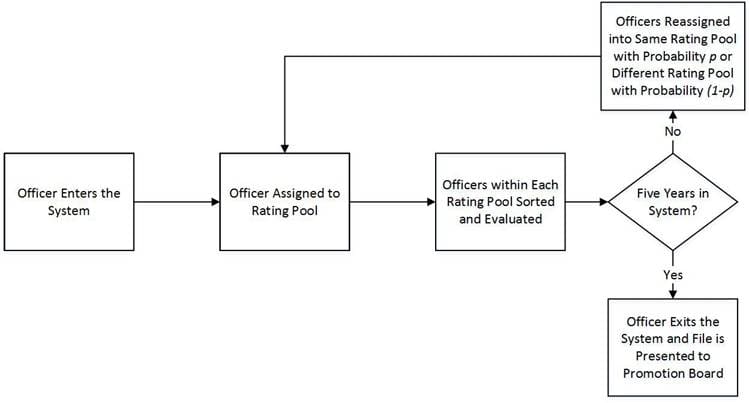
Officers receive evaluations at each assignment where they are rated relative to their peers, or officers of the same rank. Figure 2 shows the typical flow chart for a U.S. Army officer. Officers enter the evaluation system and are assigned into a group of their peers, known as a rating pool. In general, each officer is given an annual evaluation based on their performance relative to the other officers in the same rating pool. After the evaluation, the officer either remains in the same pool or is reassigned to a different pool. The reassignment typically involves a physical change in geographic location. Once an officer has spent a specified time in the system, five years in the case of Figure 1, he/she exits the system. The officer’s file is presented to a promotion board, comprised of general officers, who make the decision as to whether the officer continues to the successive rank or is forced to leave military service.

Raters are restricted from giving more than 49% of the officers in their pool a top evaluation. The intent of this forced distribution mandate is to provide a differentiation of performance for personnel management decisions. Forced distribution performance appraisal systems applied to a small number of employees create misidentification of performance. Mohrman, Resnick-West, and Lawler (1989) state that forced distribution systems should only be applied to a large enough group of individuals,  specifically   no less than 50 employees. The binomial distribution provides some insight when attempting to quantify this misidentification of performance. If X is a random variable denoting the number of top 49% per- forming officers within a rating pool of n officers, and officer performance is independent, then X follows Binomial(n, 0.49). Misidentification occur when the number of officers deserving top evaluations exceeds the profile constraint.  For example,  if n = 15,  E[Misidentifications] is ∑15, x=8  P(X = x)(x − 7) = 0.9470. When n = 100, E[Misidentifications] is ∑100, x=50   P(X = x)(x − 49) = 1.9893.  Therefore, if a population of 300 officers is divided into 20 rating pools, we would expect 18.9405 (0.9470 x 20) misidentifications. The same 300 officers divided into three rating pools results in 5.9680 (1.9893 x 3) expected misidentifications. Other factors that affect the accuracy of evaluations are the distribution of rating pool sizes, frequency of moves between rating pools, and human behavior within the system. These factors applied over a multi-year timeframe necessitate the use of techniques such as simulation to quantify the error induced by a forced distribution performance evaluation system.

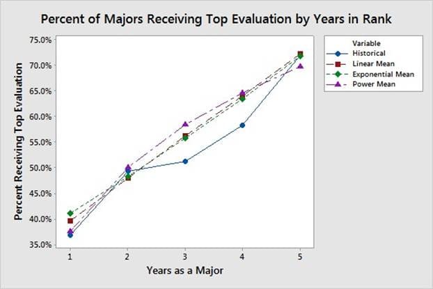
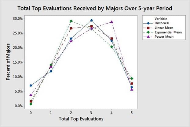
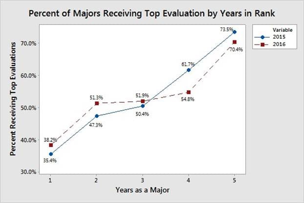
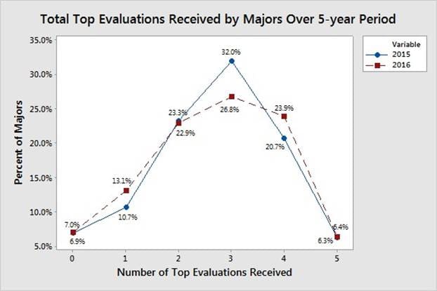
Quantifying rater behavior of ranking and evaluating subordinates requires the application of advanced model validation methods.  Figure 3 shows that officers are more likely to receive a top evaluation as  their time in rank increases. Figure 4 shows the distribution of the number of top evaluations that majors receive over a 5-year period.  The simulation output corresponding to the distributions shown in Figure    3 and Figure 4 is subject to the rater function used to rank and evaluate subordinates within each rating pool, i.e., a black-box function. The data shown in Figure 3 and Figure 4 is from majors facing promotion boards in 2015 and 2016, which had promotion rates of 60.4% and 60.2%, respectively. The basis for model comparison is an average of these two years due to their similarity and to focus the model on current evaluation trends.

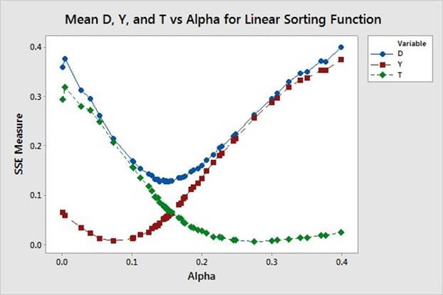
The contribution of our study is examining a method for estimating this black-box function using simulation optimization. We  build a discrete event simulation model and modify the sorting function  used to simulate human behavior using OptQuest and the Kim-Nelson (KN) procedure, a fully-sequential ranking and selection simulation optimization method. Parameters from multiple functions are evaluated to determine their goodness-of-fit in replicating rater behavior.

In order to evaluate the output, we use an adaptation of the cost function J(θ) Ikonen and Najim (2002) presented in the general form:

The quadratic cost function of Equation (1) assigns αk weights to the squared differences between K observed outputs, y(k), and the model predictions, θ T ϕ(k). The objective is to minimize the cost function J with respect to parameters θ as in Equation (2):

Section 4 elaborates on the derivation of the cost function and the parameters within the system.

Model Description

Model Input and System Dynamics

The simulation model was developed in Simio and follows the framework of Figure 2. Officers enter the system at a uniform rate and are assigned an attribute Qi that represents the officer’s initial performance percentile, where Qi Uniform(0, 1). Officers are randomly assigned into rating pools. Annually, officers are sorted and given an evaluation, Xi j where:

After each evaluation, the officer changes rating pools with probability p or remains in the same rating pool with probability 1 − p, simulating the systems dynamics of officers changing rating pools on a regular basis. Varying the value of p changes the average amount of time officers spend in each pool. A p = 0.730 corresponds to an average of 16.42 months in each position, the average time in position for officers facing promotion boards in 2015 and 2016. After five years of collecting evaluations, the officers exit the system and their binary performance appraisal history is recorded in an output file. A truncated simulation output file is shown in Figure 5.

Sorting Functions

Given the data trends in Figure 3, the proclivity for raters to award a top evaluation increases as the officers they are rating increase in seniority. Therefore, the procedure used to sort the officers uses a combination of initial performance percentile combined with a function of the time in the system. We annotate this as
Qti, where Qti(Qi,t, α), t is the officer’s time (years) in the system, and α is an estimated parameter used to apply a weight to the officer’s time in the system. Given the rater behavior, we analyze the goodness-of-fit
for the following increasing functions:

Linear: Qti  = Qi + αt                            (3)
Exponential: Qti  = Qi + αt                    (4)
Power: Qti  = Qi + tα                           (5)

Output

Figure 5 shows the simulation output for a given sorting function. The analysis of each sorting function consists of its ability to replicate the actual data shown in Figures 3 and 4. Before optimizing the parameters for each sorting function, it is necessary to determine a reasonable domain for α. For Equation (3),

An α = 0 means that rater’s determination of ranking within the rating pool is based solely off the officer’s performance percentile upon entry into the system and time in the system is not a factor. Likewise, an α = 0.4 means that the officer’s time in the system is a minimum of 0.4 times as important as Qi when t = 1 and a minimum of two times as important as Qi when t = 5 in determining the ranking within a given rating pool. Therefore, we will evaluate 0 < α < 0.4 when optimizing the output for Equation (3).

The effectiveness of Equation (4) can also be assessed using similar bounds for α. However, in Equation (4), 0 < α < 1 creates a decreasing function with respect to time in system. Furthermore, for the officer’s time in the system to carry a minimum of two times the weight of Qi  in determining the ranking within    a given rating pool for Equation (4) when t = 5, α 1.148. Therefore, we limit the domain of α for Equation (4) to 1 < α < 1.148. Similarly, we limit α in Equation (5) to 0 < α < 0.431.

Parameter Estimation

Response Function

In order to optimize the simulation output, we use a form of the multi-objective response function introduced by Ikonen and Najim (2002). The problem is formulated as:

The binary variable Zik in Equation (6) is used to identify whether each officer (i) received 0, 1, . . . , 5 top evaluations over the 5-year period in the system. Equation (7) measures the squared difference between the percentage of officers from the simulation with k top evaluations and Ak, where the variable Ak is the historical percentage of officers receiving k top evaluations. This squared error is calculated for each value of k and summed in the equation:

Equation (7) measures the goodness-of-fit of the simulation output compared to the data shown in Figure 4. The total number of top evaluations received by each officer is one measure of model accuracy. Another measure of accuracy is the timing of top evaluations each officer receives. This squared error is calculated for each year j and summed in the equation:

where B j is the percentage of officers with a top evaluation in year j. The weights, Wk  in Equation (7)  and Wj in Equation (8), allow us to control the weights of the differences between each simulation output and the actual data. This provides the ability to compensate for differences in relative error as well as the unequal number of data points in Equation (7) versus Equation (8). The value Y in Equation (8) measures the goodness-of-fit of the simulation output compared with the data shown in Figure 3.  The measures    of effectiveness provided in Equations (7) and (8) can be combined into a single weighted performance
measure, D = T + Y . Then the problem becomes finding the sorting function parameter value of α that minimizes the objective function D.  That is, αˆ  = arg min D.
α

Single Objective Parameter Estimation

To estimate the sorting function parameters, we utilize OptQuest simulation optimization routine (April, Glover, and Kelly 2002). The user has the ability to modify the minimum and maximum number of replications for a specific relative error setting, along with the maximum number of scenarios. The results from the OptQuest routine provide the list of initial candidate solutions evaluated by the KN method, a fully sequential procedure that eliminates statistically inferior solutions after each replication. We ran the KN procedure with an indifference zone of 0.001 on the best subset scenarios from the OptQuest routine in order to determine optimal setting for the parameter α in each sorting function. A detailed discussion of the KN procedure can be found in Kim and Nelson (2001). Using the Simio OptQuest add-in, 50 scenarios, with 10 replications each, took between 15 and 16 minutes to execute on an Intel@ Core i5-4300U at 2.50 GHz with 8.00 GB of RAM.

For single objective parameter estimation, we performed two separate experiments to find the parameters for each sorting function that solved:

In Equation (8), B j = [0.368, 0.493, 0.512, 0.582, 0.719], which represents the percent of majors facing promotion in 2015 and 2016 that received a top evaluation each year in rank. The parameter α was evaluated in Equations (3), (4), and (5), and the minimum Y for each sorting function is shown in Figure 6.

Given that W j = [1, 1, 1, 1, 1], Table 1 summarizes the performance of each sorting function with the optimal parameter settings. Each sorting function is compared to the best in the ”Percent Gap” column in Table 1.

Table 1: A summary of the minimum Y for each sorting function with α determined by simulation optimization.

The parameter α was also evaluated in Equations (3), (4), and (5) and the minimum T for each sorting function is shown in Figure 7. In Equation (7), Ak = [0.070, 0.119, 0.231, 0.294, 0.223, 0.064], which represents the historical percentages of officers facing promotion in 2015 and 2016 that received [0, 1,…,5] total top evaluations as a major. Given that Wk = [1, 1, 1, 1, 1, 1], the minimum T for each sorting function and a comparison of each sorting function with the best is shown in Table 2.

Table 2: A summary of the minimum T for each sorting function with α determined by simulation optimization.

Weighted Multi-Objective Parameter Estimation

In the single objective parameter estimation, we used separate equations for each sorting function when determining the minimum T and Y . For the multi-objective parameter estimation, we used a weighted sum of Y and T . Thus, it is necessary to determine appropriate W j and Wk for the response function, D. Equation (8) sums the squared error between six simulation outputs and historical data, whereas  Equation (7) sums the squared error between five data points and historical data. Therefore, we begin by setting each component of Wk to 5/6 in order weight the outputs of T and Y equally. Finally, we factor relative error into Wk. The mean value of the responses used in Equation (7) is 0.535, representing the average percentage of majors receiving a top evaluation in any given year. The mean value of the responses used in Equation (8) is 0.167, representing the average percentage of majors receiving each of the six possibilities for a total number of top evaluations. We compensate for the difference in magnitudes by multiplying the initial Wk by 3.21 (0.535/0.167) and each component of vector Wk is 2.675 (3.21 5/6). Therefore, when evaluating D, we use W j = [1, 1, 1, 1, 1] and Wk = [2.675, 2.675, 2.675, 2.675, 2.675, 2.675]. Figure 8 shows that minimizing D does not minimize Y or T .

The efficacy of our weighted multi-objective approach is illustrated in the two graphs of Figure 9. The line labeled “No Time Factor” represents a static performance level with no added time factor, resulting in D = 0.864. The tradeoff between T and Y shown in Figure 8 results in a decreased percent improvement from the single-objective parameter estimation responses summarized in Tables 1 and 2. Table 3 shows the value of D using the optimal parameter settings for each of the three sorting functions.

Table 3: A summary of the minimum D for each sorting function with α determined by simulation optimization.